Recurrent Neural Networks
Introduction:
One of the most plausible analogy for RNNs
Humans don’t start their thinking from scratch every second. As you read this essay, you understand each word based on your understanding of previous words. You don’t throw everything away and start thinking from scratch again. Your thoughts have persistence.
Traditional neural networks can’t do this, and it seems like a major shortcoming. For example, imagine you want to classify what kind of event is happening at every point in a movie. It’s unclear how a traditional neural network could use its reasoning about previous events in the film to inform later ones.
Recurrent neural networks address this issue. They are networks with loops in them, allowing information to persist.
What is RNN?
A recurrent neural network is a neural network that is specialized for processing a sequence of data (t)= x(1), . . . , x(τ) with the time step index t ranging from 1 to τ. For tasks that involve sequential inputs, such as speech and language, it is often better to use RNNs. In a NLP problem, if you want to predict the next word in a sentence it is important to know the words before it.
RNNs are called_recurrent_because they perform the same task for every element of a sequence, with the output being depended on the previous computations. Another way to think about RNNs is that they have a “memory” which captures information about what has been calculated so far.
Basics: – recurrent neural network is that it is capable of emulating some primitive form of memory
consider the two sentences
“I went to Nepal in 2009”
and
“In 2009,I went to Nepal.”
If we ask a machine learning model to read each sentence and extract the year in which the narrator went to Nepal, we would like it to recognise the year 2009 as the relevant piece of information Ian GoodFellow Chapter 10
h(t) = f(h(t−1), x(t); θ)
is the general equation of the RNN structure. /( unrolls over time /)
–> When the recurrent network is trained to perform a task that requires predicting the future from the past, the network typically learns to use h(t) as a kind of lossy summary of the task-relevant aspects of the past sequence of inputs up tot. This summary is in general necessarily lossy, since it maps an arbitrary length sequence (x(t), x(t−1), x(t−2), . . . , x(2), x(1) to a fixed length vector h(t).
For example, if the RNN is used in statistical language modeling, typically to predict the next word given previous words, storing all the information in the input sequence up to time t may not be necessary; storing only enough information to predict the rest of the sentence is sufficient. The most demanding situation is when we ask h(t)to be rich enough to allow one to approximately recover the input sequence, as in autoencoder 370
However, there are certain problems with RNN which gave birth to LSTM , Gated networks which we’ll discuss later.
Coming back to RNNs.
Sequential processing in absence of sequences even if your data is not in form of sequences, you can still formulate and train powerful models that learn to process it sequentially. You’re learning stateful programs that process your fixed-sized data.
Architecture :
Let us briefly go through a basic RNN network.
Input:
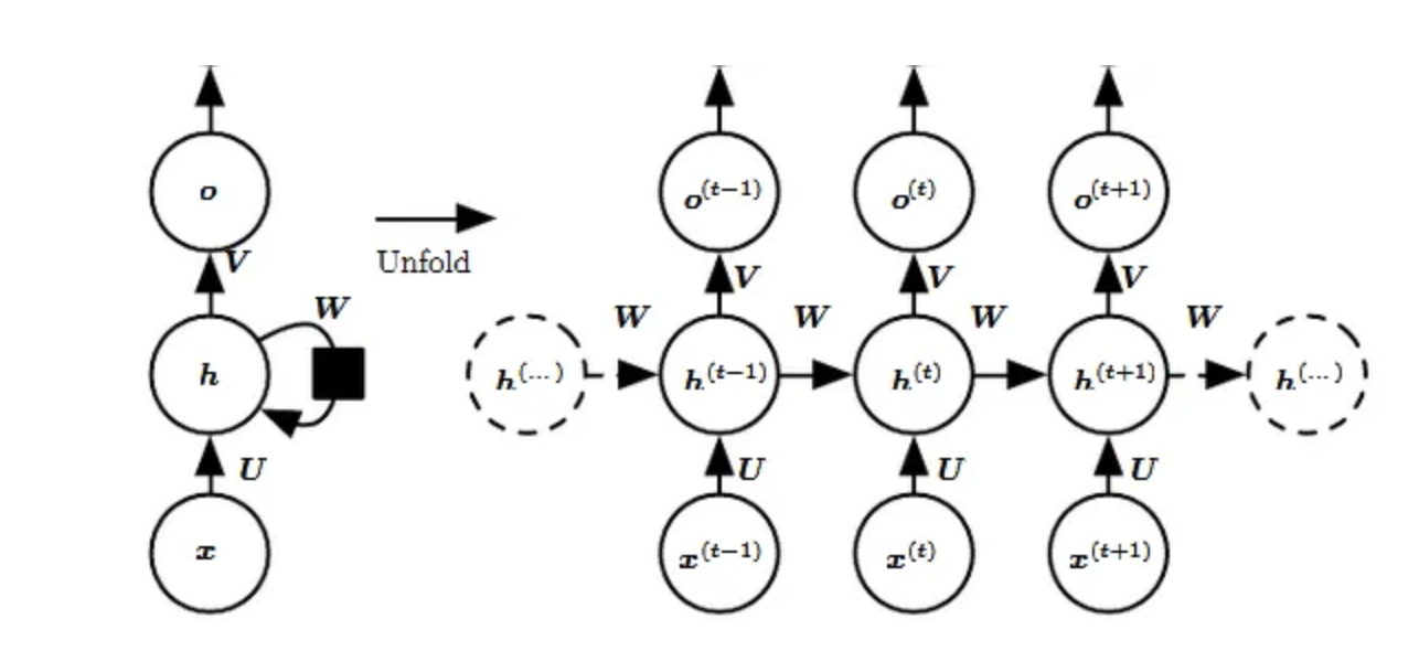
x(t) is taken as the input to the network at time step t. For example, x1, could be a one-hot vector corresponding to a word of a sentence.
Hidden state:
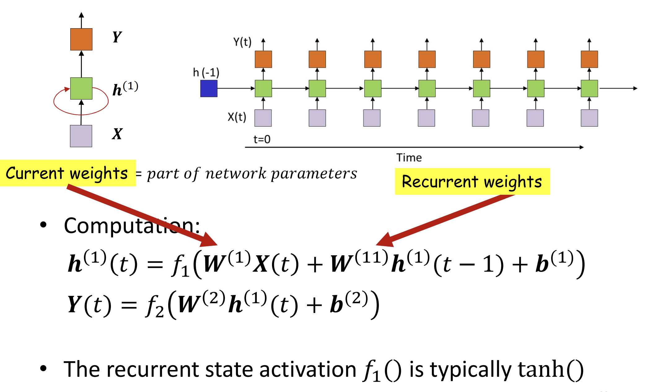
h(t) represents a hidden state at time t and acts as “memory” of the network. h(t) is calculated based on the current input and the previous time step’s hidden state:
h(t) = f(U.x(t) + W .h(t−1)).
The function f is taken to be a non-linear transformation such as tanh, ReLU.
Weights:
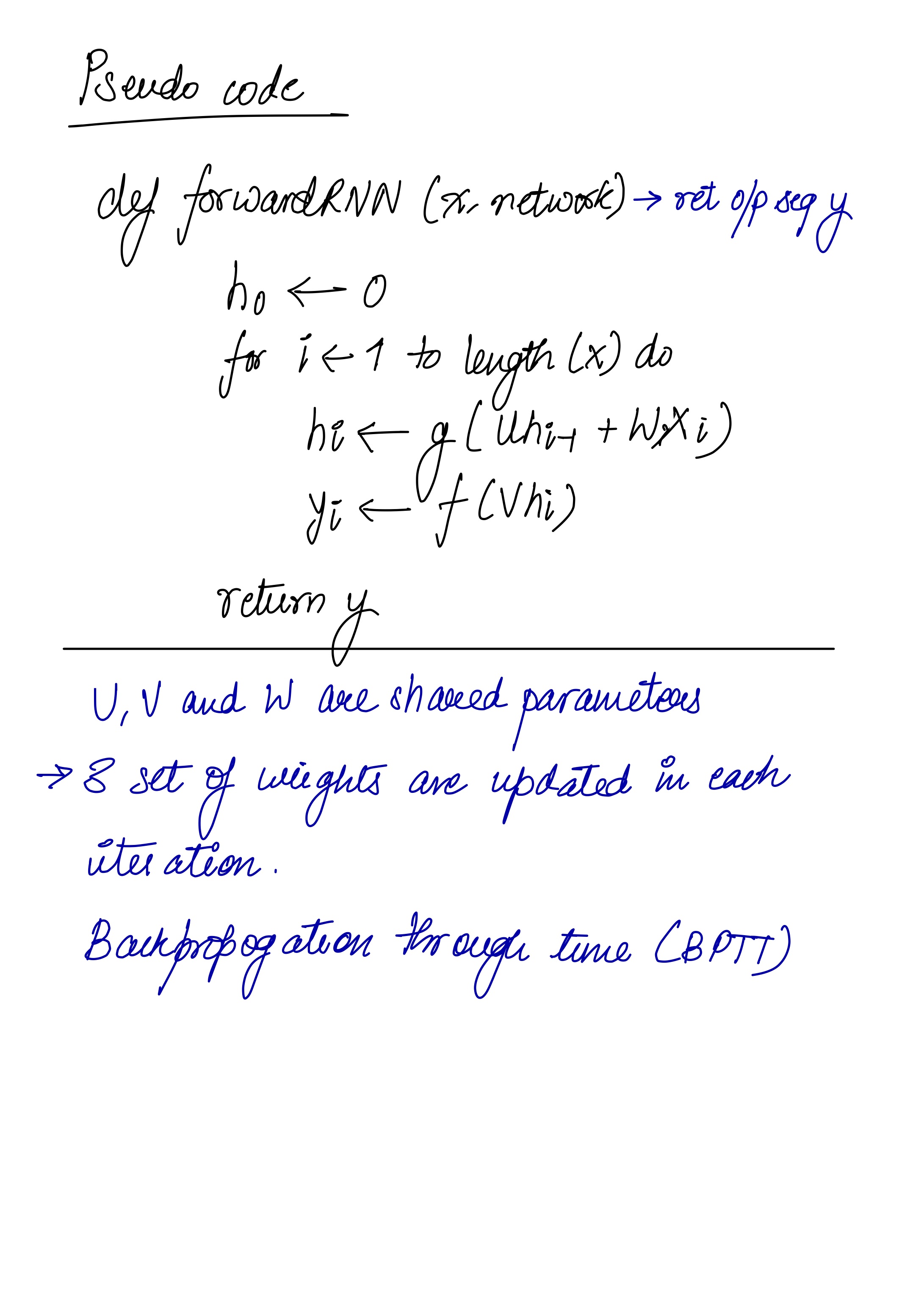
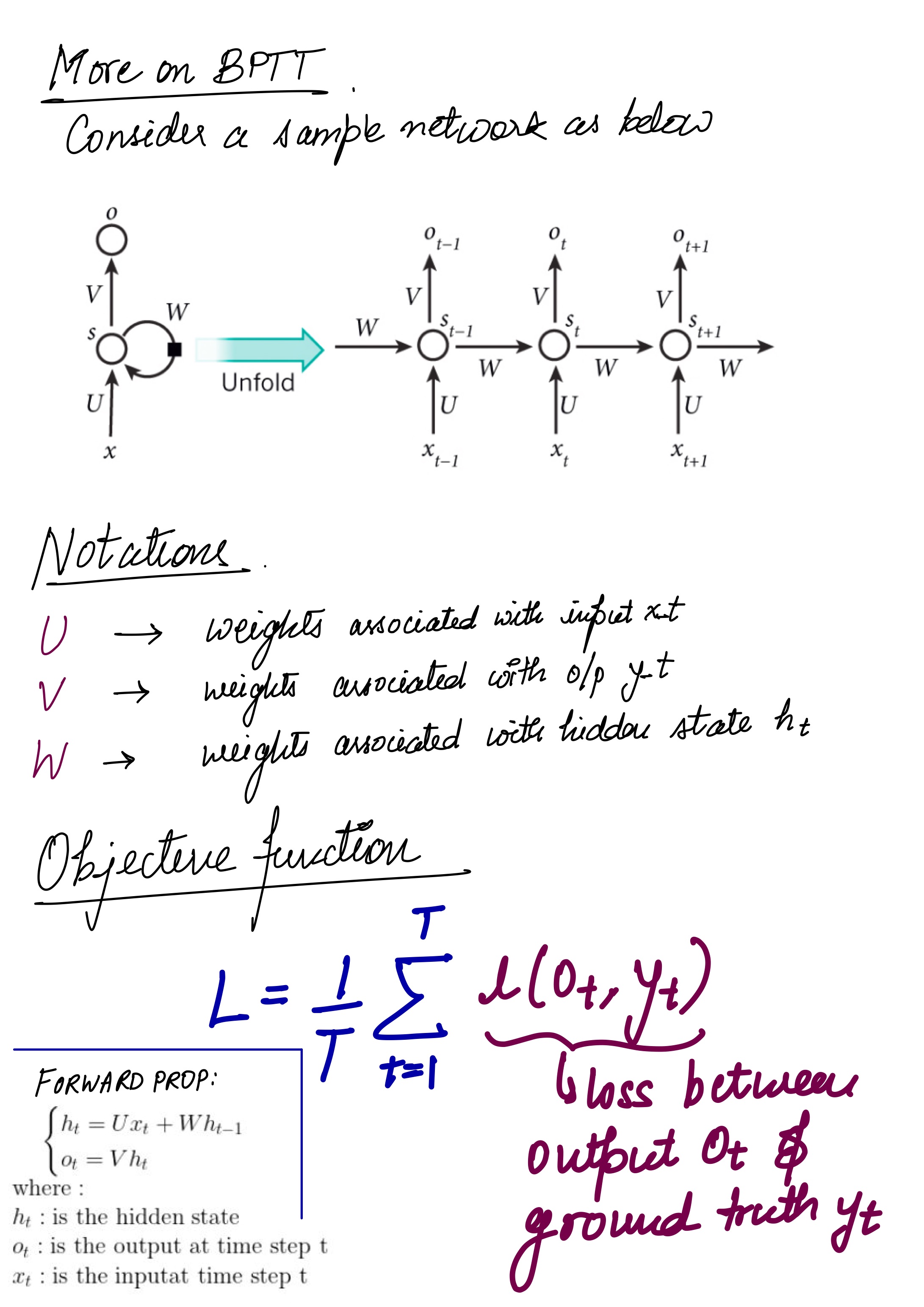
The RNN has – input to hidden connections parameterised by a weight matrix U, – hidden-to-hidden recurrent connections parameterised by a weight matrix W, – and hidden-to-output connections parameterised by a weight matrix V and all these weights (U,V,W) are shared across time.
Output:
o(t) illustrates the output of the network. In the figure I just put an arrow after o(t) which is also often subjected to non-linearity, especially when the network contains further layers downstream.
Forward Pass
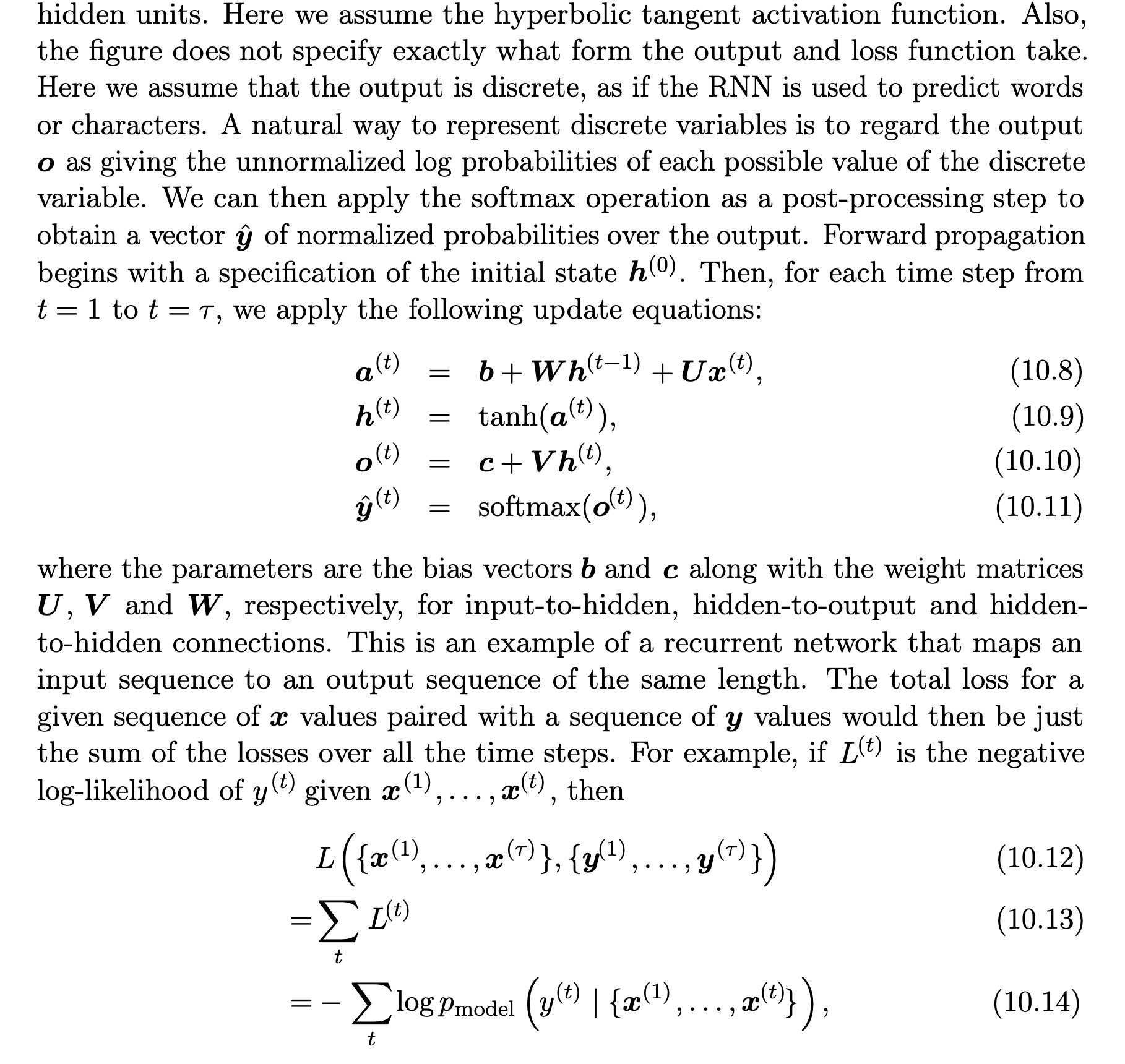
The figure does not specify the choice of activation function for the hidden units. Before we proceed we make few assumptions: 1) we assume the hyperbolic tangent activation function for hidden layer. 2) We assume that the output is discrete, as if the RNN is used to predict words or characters. A natural way to represent discrete variables is to regard the output o as giving the normalised log probabilities of each possible value of the discrete variable. We can then apply the softmax operation as a post-processing step to obtain a vector ŷ of normalised probabilities over the output.
The RNN forward pass can thus be represented by below set of equations.
This is an example of a recurrent network that maps an input sequence to an output sequence of the same length. The total loss for a given sequence of x values paired with a sequence of y values would then be just the sum of the losses over all the time steps. We assume that the outputs o(t)are used as the argument to the softmax function to obtain the vector ŷ of probabilities over the output. We also assume that the loss L is the negative log-likelihood of the true target y(t)given the input so far.
Backward Pass
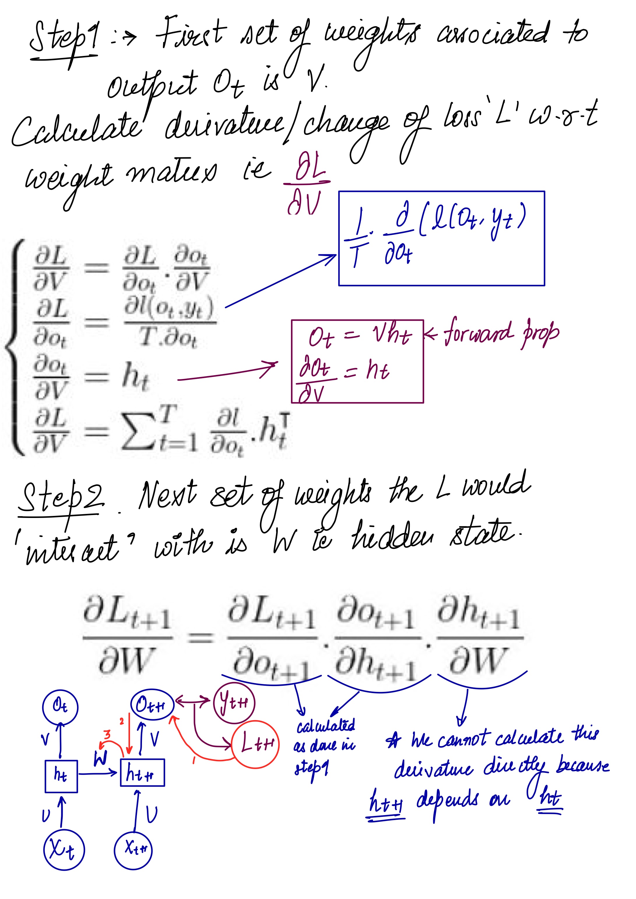
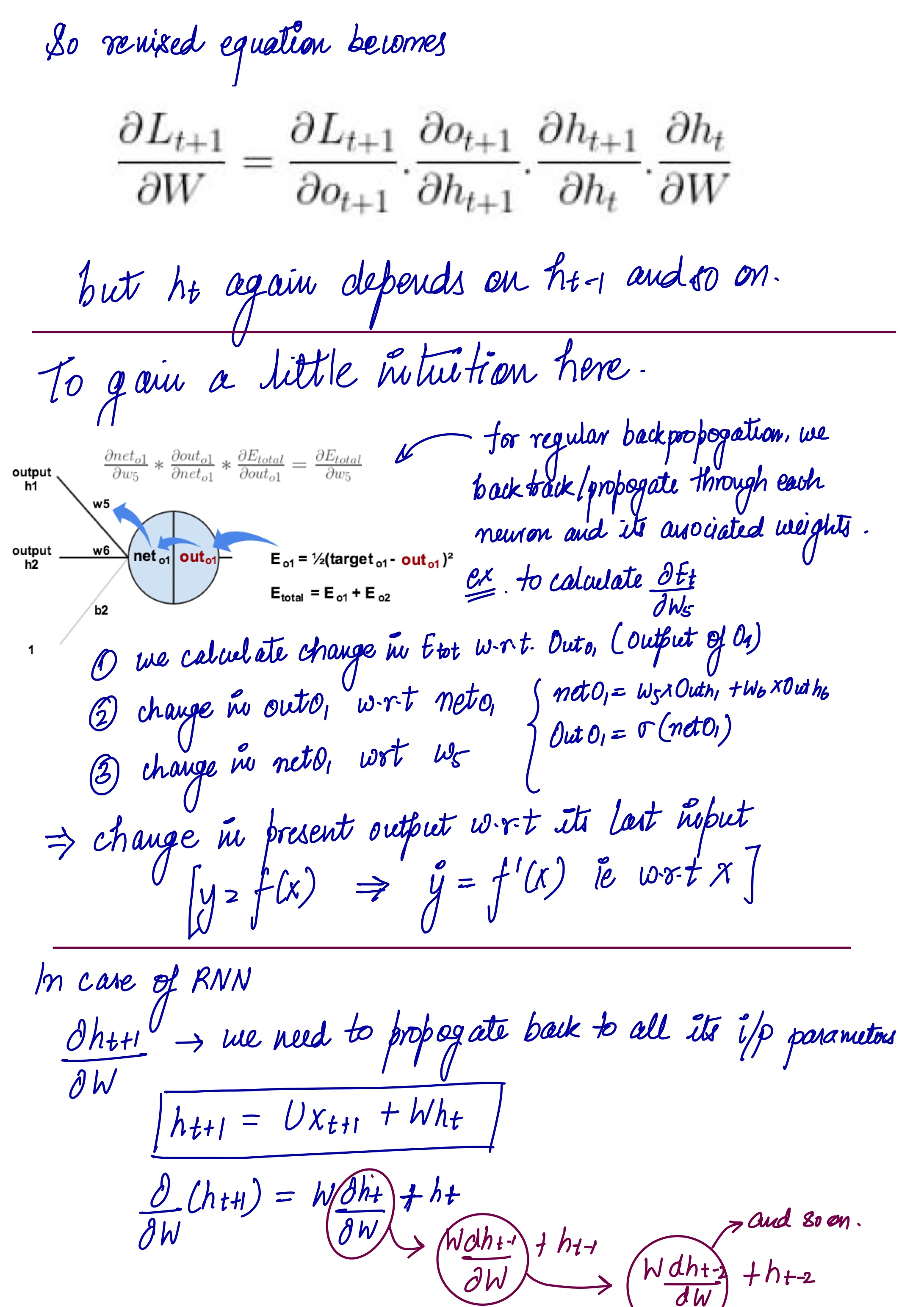
The gradient computation involves performing a forward propagation pass moving left to right through the graph shown above followed by a backward propagation pass moving right to left through the graph. The runtime is O(τ) and cannot be reduced by parallelization because the forward propagation graph is inherently sequential; each time step may be computed only after the previous one. States computed in the forward pass must be stored until they are reused during the backward pass, so the memory cost is also O(τ). The back-propagation algorithm applied to the unrolled graph with O(τ) cost is called back-propagation through time (BPTT). Because the parameters are shared by all time steps in the network, the gradient at each output depends not only on the calculations of the current time step, but also the previous time steps.
Computing Gradients
Given our loss function L, we need to calculate the gradients for our three weight matrices U, V, W, and bias terms b, c and update them with a learning rate α. Similar to normal back-propagation, the gradient gives us a sense of how the loss is changing with respect to each weight parameter. We update the weights W to minimise loss with the following equation: W = W - α * (∂L / ∂W)
The same is to be done for the other weights U, V, b, c as well. now compute the gradients by BPTT for the RNN equations above. The nodes of our computational graph include the parameters U, V, W, b and c as well as the sequence of nodes indexed by t for x (t), h(t), o(t) and L(t). For each node n we need to compute the gradient ∇nL recursively, based on the gradient computed at nodes that follow it in the graph.
Gradient with respect to output o(t) is calculated assuming the o(t) are used as the argument to the softmax function to obtain the vector ŷ of probabilities over the output. We also assume that the loss is the negative log-likelihood of the true target y(t).
–> Chapter 10 for more on BPTT on each weight matrix.
Few notes on BPTT from CMU notes:
Divergence between output (o(t)) and y(t) do not have one to one correspondence which kind of make sense. For eg in speech translation, from English to Hindi, not every word of English is going to be mapped to each word of desired sequence in Hindi. So we can’t calculate loss for each time=t Loss(t) = y(t) - o(t)
As a convenience measure, The total loss for a given sequence of x values paired with a sequence of y values would then be just the sum of the losses over all the time steps.(we assume one to one correspondence here) For example, if L(t) is the negative log-likelihood of y(t) given x(1), . . . , x(t) , then
A nice visualisation of RNN –> RNN_visualisation
-> Each cell is unrolled over time ( consider it like a for loop with sharing weights ).
Scary Mathematical equations for a toy RNN ( While writing this I discovered these are called ‘Vanilla RNNs’ :P , fancy name though )
Step1: Calculation of current hidden state h(t) Hidden state at any given point of time is an affine function of the (current input x(t)) and (previous hidden state (h{t-1}) ) plus bias which again goes through an activation fcuntion f1
Step2: Calculation of current output y(t): Current output is calculated as an affine function of current state + bias
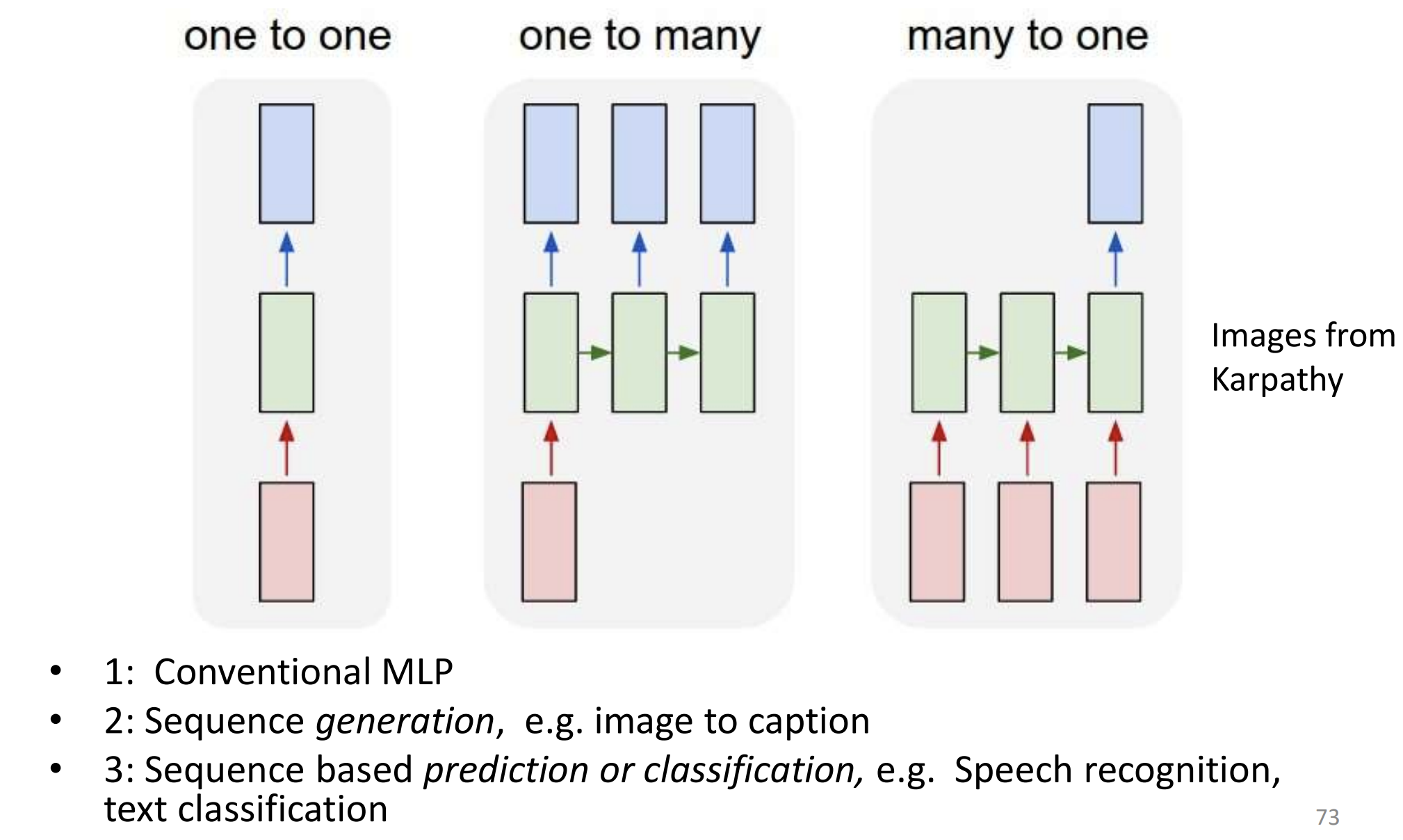
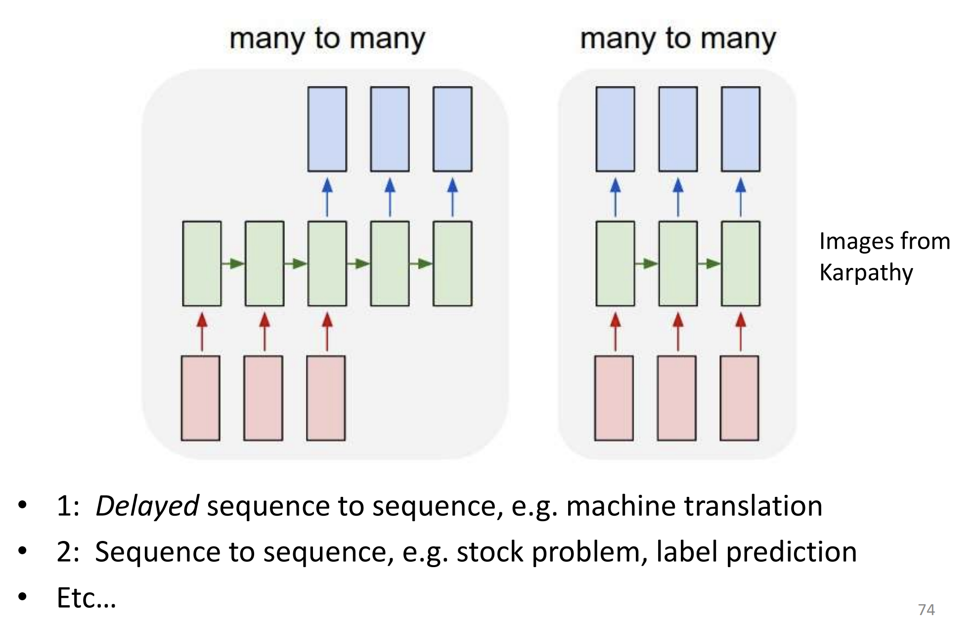
Variants of RNNS:
Pseudo code for the forward step:
Let’s build one from scratch:
Step1: Create basic RNN class:
1
2
3
4
5
6
7
8
9
10
11
12
13
14
class RNN():
    def __init__(self, x, y, hidden_size):
        self.x =x
        self.y =y
        self.hidden_units = hidden_size

        # Let's define weight paramters ( U, V and W)
        '''What will be the shape of these weights?
        '''
        self.U = None
        self.V = None
        self.W = None
        self.b = None
        self.c = None
A note on weight initialisation: Proper initialisation of weights seems to have an impact on training results there has been lot of research in this area. It turns out that the best initialisation depends on the activation function (tanh in our case) and one recommended approach is to initialise the weights randomly in the interval from[ -1/sqrt(n), 1/sqrt(n)]where n is the number of incoming connections from the previous layer.
Remember weight U is multipled with X , W is multipled with h(t-1) and V is for output .
Forward loop:
1
2
3
4
5
6
7
8
9
10
11
12
13
14
15
16
17
18
19

        def forward(self,input,hprev):
            '''
            This is simple
            '''
            xs,hs,os,ycap={},{},{},{}
            hs[-1] = np.copy(hprev)
            for t in range(len(inputs)):

                xs[t] = zero_init(self.vocab_size,1)
                xs[t][inputs[t]] = 1
				hs[t] = np.tanh( np.dot(self.U, xs[t]) + np.dot(self.W, hs[t-1]) +self.b  )
                os[t] = np.dot(self.V,hs[t]) + self.c
                ycap[t] = self.softmax(os[t])
            return xs, hs, ycap

        def loss(self,ps,targets):
            #This should be negative likelihood as in Goodfellow chapter 10
            return np.sum( -np.log(ps[t][targets[t],0]) for t in range(self.seq_length) )
BPTT:
1
2
3
4
5
6
7
8
9
10
11
12
13
14
15
16
17
18
19
20
21
22
23
24
25
26
27
28
29
30
31
32
33
34
35
36

''''
        TRicky part (BPTT)
        '''
        def backward(self, xs, ps, ycap, targets):
            dU, dW, dV = np.zeros_like(self.U), np.zeros_like(self.W), np.zeros_like(self.V)
            dB, dC = np.zeros_like(self.b), np.zeros_like(self.c)

            dhNext  = np.zeros_like(hs[0])

            for t in reversed(range(self.seq_length)):

                dy = np.copy(ps[t])

                dy[target[t]]-=1

                dV+=np.dot(dy, hs[t].T)
                dC+=dC

                dh = np.dot(self.V.T, dy) + dhNext

                dhrec = ( 1 - hs[t]* hs[t]) *dh
                dV + =dhrec

                dU + =np.dot(dhrec,xs[t].T)
                dW+ = np.dot(dhrec,hs[t-1].T)


                dhNext = np.dot(self.W.T, dhrec)

            for dparam in [dU, dW, dV, db, dc]:
                np.clip(dparam, -5, 5, out=dparam)
            return dU, dW, dV, db, dc

            '''Woah!!!
            '''
Problems with RNN:
The runtime is O(τ) and cannot be reduced by parallelisation because the forward propagation graph is inherently sequential; each time step may be computed only after the previous one. States computed in the forward pass must be stored until they are reused during the backward pass, so the memory cost is also O(τ).
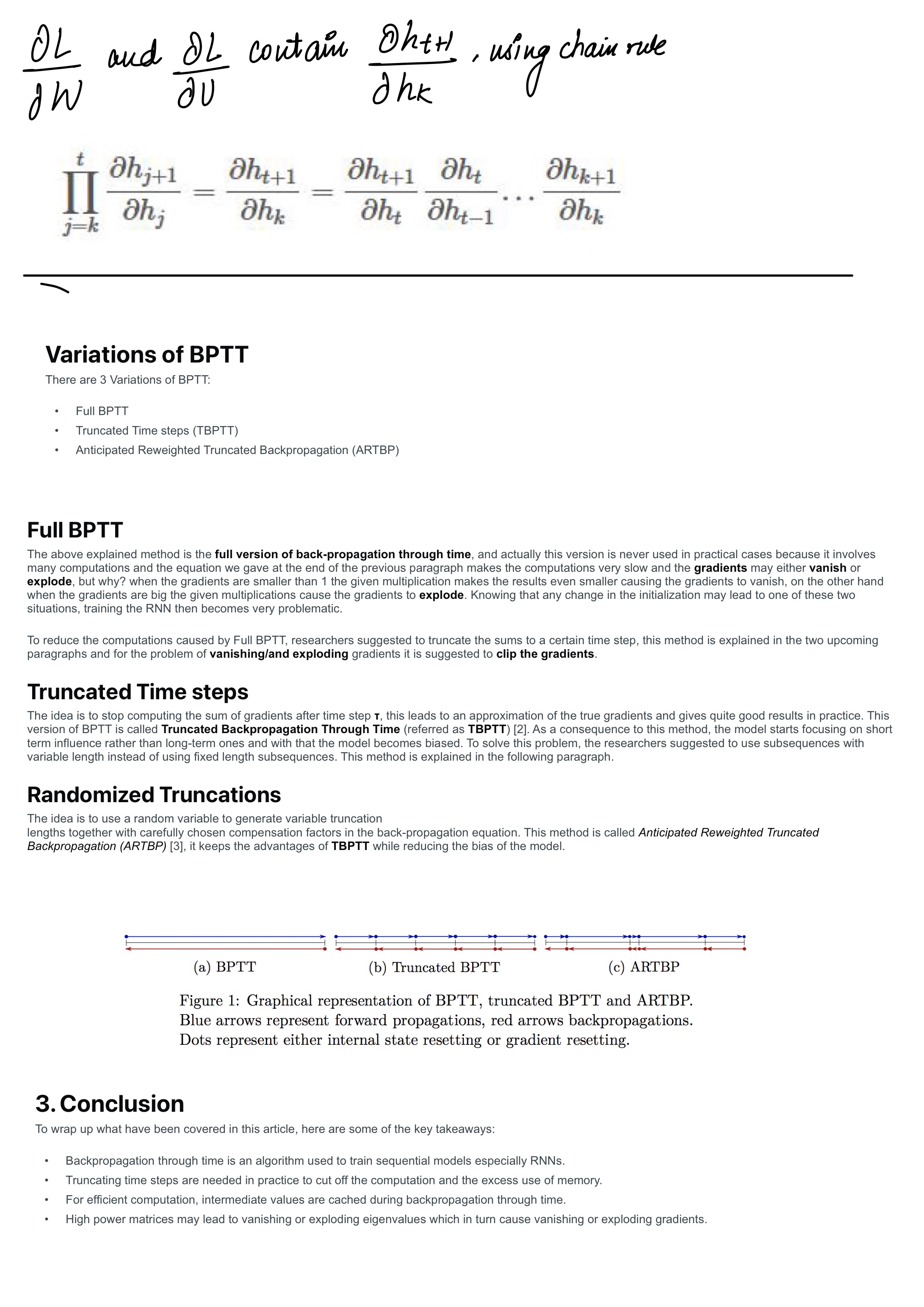
Also, The above explained method is the full version of back-propagation through time, and actually this version is never used in practical cases because it involves many computations and the equation we gave at the end of the previous paragraph makes the computations very slow and the gradients may either vanish or explode, but why? when the gradients are smaller than 1 the given multiplication makes the results even smaller causing the gradients to vanish, on the other hand when the gradients are big the given multiplications cause the gradients to explode. Knowing that any change in the initialization may lead to one of these two situations, training the RNN then becomes very problematic.
Knowledge Gaps remaining:
BPTT and its matrix implementation. Jacobian and all
Update: 21th July,2023
Sources


-1.jpg)
-2.jpg)

